Posts
Least squares, three ways
The normal equations, QR, and the SVD solve the same problem with very different accuracy. The difference is the square of a condition number.
Linear least squares asks for the coefficients that minimize for a tall matrix . Setting the gradient to zero gives the normal equations,
and in NumPy they take one line:
beta = np.linalg.solve(X.T @ X, X.T @ y)That line is short, fast, and the least accurate of the three standard methods. This note measures how much accuracy it gives up, explains why, and says when the loss does not matter.
An experiment with a known answer
#Polynomial fitting is the classic way to make a least-squares problem hard. On equally spaced points , the columns of the monomial basis look more and more alike as grows, and the matrix drifts towards rank deficiency.
To isolate the solver, I chose the right-hand side so that the exact solution is known: and , with a residual of zero. Any error in then comes from floating-point arithmetic, not from the data.
import numpy as np

def errors(p, m=100):
    t = np.linspace(0.0, 1.0, m)
    X = np.vander(t, p, increasing=True)
    beta = np.ones(p)
    y = X @ beta
    rel = lambda b: np.linalg.norm(b - beta) / np.linalg.norm(beta)

    normal = np.linalg.solve(X.T @ X, X.T @ y)
    Q, R = np.linalg.qr(X)
    qr = np.linalg.solve(R, Q.T @ y)
    svd = np.linalg.lstsq(X, y, rcond=None)[0]
    return np.linalg.cond(X), rel(normal), rel(qr), rel(svd)
np.linalg.qr computes a Householder factorization, and np.linalg.lstsq calls LAPACK’s SVD-based solver. The relative errors in the coefficients:
| Columns | Condition number | Normal equations | QR | SVD |
|---|---|---|---|---|
| 4 | ||||
| 6 | ||||
| 8 | ||||
| 10 | ||||
| 12 |
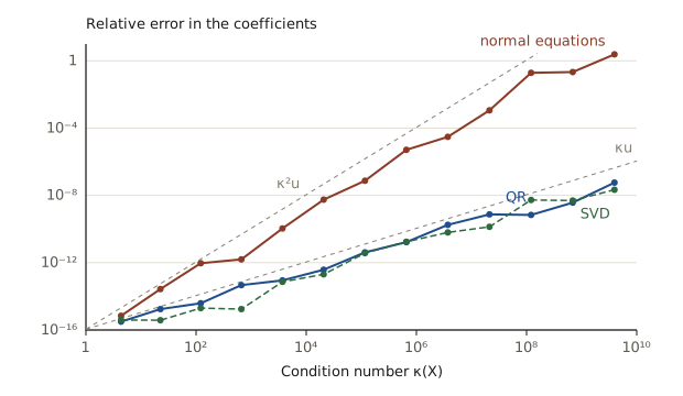
With twelve columns the normal equations return coefficients that are wrong in the first digit, while QR and the SVD still agree with the truth to eight or nine digits. Plotting every from 2 to 14 against the condition number shows two straight lines with different slopes.
Why the normal equations lose twice as many digits
#The condition number measures how much a matrix can amplify relative perturbations. Forming squares it.
A backward-stable solver for a square system with matrix returns a solution with relative error of order , where is the unit roundoff of double precision. Solving the normal equations is such a solve with . Householder QR and the SVD never form that product: they work on itself, and for a problem with a small residual their error is of order .1
The estimates are upper bounds up to modest constants, and the measured errors sit at or below the dashed guides in the figure. Each factor of ten in costs QR about one decimal digit and the normal equations about two.
When the residual is large, even the best algorithm inherits a term proportional to times the relative size of the residual. That term belongs to the problem, not to the method, so no choice of solver removes it.2
When the normal equations are fine
#None of this makes the normal equations wrong. They are the right tool more often than the table suggests.
- The matrix is well conditioned. With , the normal equations lose about four digits and still deliver twelve. Standardized predictors with little collinearity are often in this range.
- The data do not fit in memory. and can be accumulated in one pass over the rows, in storage, and solved at the end.
- Speed matters more than the last digits. For , forming costs about operations; Householder QR costs about .
Change the basis before changing the solver
#The cheapest fix is often in the model rather than the algorithm. The monomials on are a notoriously poor basis. Moving the same points to brings the condition number of the twelve-column matrix from down to , and a Chebyshev basis on brings it to . At that point all three methods agree to the last digit, and the normal equations are as good as any.
The general lesson is that accuracy is decided twice: once when the problem is posed, by the condition number, and once when it is solved, by whether the algorithm squares it.
Lloyd N. Trefethen and David Bau III, Numerical Linear Algebra (SIAM, 1997), Lectures 18 and 19, analyse the conditioning of least-squares problems and the stability of these three algorithms. ↩︎
Nicholas J. Higham, Accuracy and Stability of Numerical Algorithms, 2nd edition (SIAM, 2002), Chapter 20, gives the perturbation theory, including the residual term. ↩︎